Modern computer systems are quite fascinating. They are highly complex, run a lot of software, and their performance characteristics are hard or impossible to predict.
Earlier this year, I gave a lecture on benchmarking, which for lack of generic and always-applicable advice, I started with a brainstorming session about its pitfalls. Since systems have become so complex that we rarely know what happens exactly. We are prone to simply guess whatâs going on. Or rather, we should hypothesize and verify our hypothesis. Still, there might be many more causes for what we see than we can initially think of.
To illustrate this, Iâll use some fictitious benchmark results,
which are fairly close to what one would see in reality,
and there are usually many possible explanations
for the observed behavior.
This often means, only once we know what caused a specific artifact,
we can make progress with understanding what we set out to understand in the first place.
The Scenario: A âReasonably Deterministicâ Workload
Letâs start with our hypothetical/fictitious benchmark. One rather strong assumption we are going to make is that our benchmark is âreasonably deterministicâ. Thus, when we run it multiple times, it pretty much does the same thing. To make this more concrete, letâs assume our benchmark does what one of the very first business applications did: payroll. We have a program that generates PDFs with the monthly payslips. We run our benchmark on a Linux from 2026 and since our hypothetical benchmark is written in Java, we use the HotSpot JVM and JDK 26.
A First Run
We let this benchmark run for 8 iterations within the same JVM process and visualize all our data points with a scatter plot. On the y-axis we show run time, which means lower is better. On the x-axis, we have the number of the specific iteration.
On the plot we can see that iterations 2, 3, 4 are each a bit faster than the previous one, and then we stay at the same level of performance.
Given that we use a language implementation with just-in-time (JIT) compilation, this is what we would roughly expect. The JIT compiler manages to optimize the code we are executing step by step, and we see that it improves performance.
A Second Run, Same Benchmark, Nothing Changed
We ran the exact same setup a second time, getting 8 new data points. But as we can see in Figure 2, the benchmark is faster in iteration 3 and following! What happened here?
This is where we now start hypothesizing.
What could it be?
It could be that the operating system decided
to give it different physical memory,
or run it on a different kind of core (many CPUs these days have 2 or more different types of cores with different performance).
Perhaps, we ran out of thermal budget and the CPU ran at a lower clock speed to
avoid overheating?
Or, since we are on a JVM,
perhaps the compiler saw slightly different information for the types/behavior
seen in the first and second iterations, and thus, made slightly different optimization decisions?
This is possible because compilation happens on a background thread, and thus,
even when the benchmark is deterministic, the used profiling information is to some degree racy.
It could also be something entirely different however, which means, we do not really know.
For designing your benchmark methodology,
youâll need to decide on how to take these variables into account.
Sometimes, you may simply collect data from more runs, ideally many runs,
so that you can characterize this behavior as part of the
performance distribution one might likely observe in practice.
In other cases, this might be too naive, and you need to carefully control
for specific variables to get useful data from your experiments.
This can include pinning threads to specific cores, fixing CPU frequencies,
disabling address space layout randomization, etc. Each approach comes with different
tradeoffs.
A Third Run, And More Data
We ran the same benchmark, with the very same setup, a third time. And, we actually had a few more than the 8 data points I showed before.
The third run was slower. What happened now? Still guessing, we could assume
we simply didnât get as lucky as the second time. Indeed, we might have gotten
rather unlucky, at least until iteration 14.
So, the same mechanisms that made the second run faster, could have now played
against us, and made the third run slower.
And thatâs why performance is a distribution.
But, at iteration 15, something else happened in addition.
This isnât a change between runs, i.e., a change between different operating system
processes. Itâs a change within the same process, and after performance already looked stable.
Indeed, this might be something that happened hours, not minutes, after we thought that performance is stable. We could still be guessing that it is very much the same mechanisms as before though. The operating system may just have decided our workload needs to be handled somehow differently: different core, different core type, different physical memory, etc.
Or it could have been a mechanism somewhere else in the software stack that changed based on some heuristic that triggered only after that time. And indeed, there are various mechanisms hiding. Colleagues saw behavior like this in the JVM, where it would free classes generated internally by the JVM to speed up reflection. The JVM sets a timeout based on the maximum heap size. Using 1 second per MB of heap, which can mean it happens very late in an experiment. Go, read their Experimental Evaluation Methodology for the Era of No Steady Performance paper, itâs a fun read.
Same Benchmark, Different Input
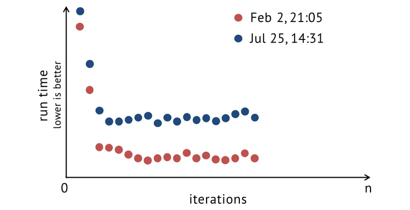
Letâs look at one more set of fictitious results.
This time, we see a more irregular pattern. Though, we still see a major performance difference between the two runs.
Our hypotheses might include all of the above, but perhaps additionally, it could include garbage collection (GC) more generally. We see a bit of an up and down. So, perhaps the GCs are not fully part of every iteration, as we might guess compared to the previous plots. Thus, here we might see the impact of the JVMâs garbage collector.
But, it could also be something about the dates at which the experiments ran.
Did we run this on a laptop? Was it plugged into power in the past, and now isnât, or the other way around? Was it cold in February, and now itâs hot, so, the CPU clocks itself down? Did we update the software between these runs?
It really could be a million different things.
All we know is that it is probably not safe to assume that the data is comparable. And thatâs really the one thing we always need to investigate: Are we confident that the data we obtained is comparable, or has some hidden variable changed that we did not account for?
Pitfalls When Benchmarking
When benchmarking, there are unfortunately a lot of things we may need to consider. Some of them, we can find ways to account, i.e., control for. Though, thatâs at the risk of reviewers saying that the setup is unrealistic. (Iâd argue, explainability trumps realism in many cases.) Other pitfalls, we might only be able to address by collecting more data. And yet others might mean we need to start all over again.
Since this is a rather complex area, I do not have any quick and simple solutions. So, letâs conclude with my incomplete overview of things to keep in mind:
- Run-time optimizations
- Feedback-based compiler decisions
-
Memory changes, garbage collection
-
Security mechanisms
- Address space layout randomization
-
Hardware complexity
- Memory hierarchies, caches, locality
- Cores, core types, â¦
-
Dynamic clock frequency changes
- Thermal budgets -
Environmental impact
- Temperature
-
Power source
-
Software updates/changes
- Linking order
And many moreâ¦