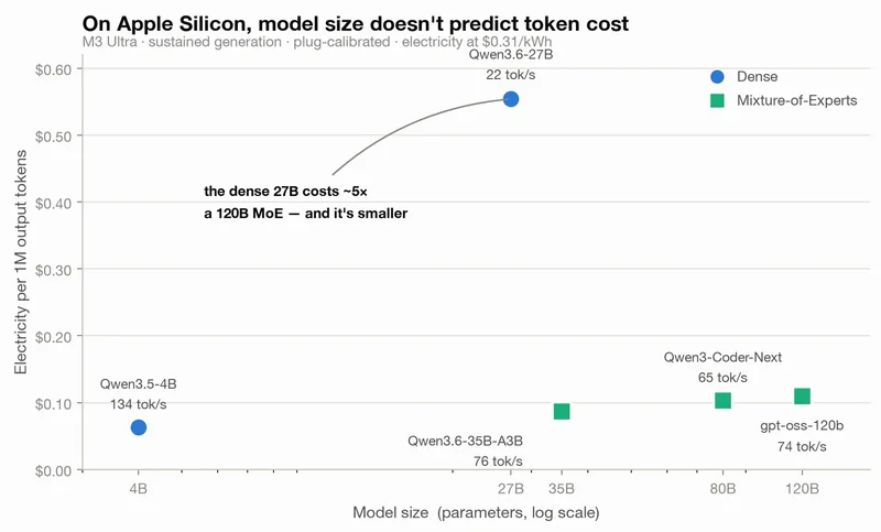
throughput, not parameter count.
I don’t have a 3090. I run everything on an M3 Ultra Mac Studio with 96 GB of unified memory—no discrete GPU, no VRAM, just one pool of memory the CPU and GPU share. That’s a different enough machine that I wanted to know whether the same surprise holds, and by how much. So I measured it. Five models, sustained generation, real wall-socket energy, priced at my actual utility rate. The short version: the surprise doesn’t just hold on Apple Silicon, it gets bigger. My 120-billion-parameter model is about five times cheaper per token than a model a quarter its size.
Here’s how I got the numbers, and why they land where they do.
How the measurement works
The instrument is a small tool I built called TokenWatt. It’s an OpenAI-compatible proxy built just for Apple Silicon: you point it at whatever local inference server you already run, and it forwards every request byte-for-byte while bracketing it with an energy measurement. It reads the whole-SoC power rails through Apple’s IOReport interface—the same counters Activity Monitor’s energy tab is built on—which means no sudo, no external instrumentation, just the numbers the chip reports about itself. It subtracts a rolling idle baseline so you’re measuring the marginal cost of the request, not the machine sitting there breathing, and it prices the result at your electricity rate. Mine is a flat $0.31/kWh.
The honesty problem with any measurement like this is that the on-die counters can drift, and there’s no way for a reader to know whether to trust them. So the one thing I insisted on—and the reason the tool exists at all—is calibration against ground truth. I ran every measurement in this article with the Mac plugged into a Shelly Plug US Gen4 that meters actual energy at the wall, and TokenWatt’s built-in calibration fit the SoC counters to it—no hand-tuning, and the same procedure anyone with a metering plug can rerun. Every number below carries a real error band from that fit; they land between ±2.6% and ±4.5%. When you see “$0.109 per million tokens,” that’s a wall-verified figure with a stated uncertainty, not a hopeful reading off an internal register.
For the headline numbers I ran each model in a sustained generation loop—the machine doing nothing but decoding tokens as fast as it can—at three durations (120, 360, and 720 seconds), three passes each, with a 15-minute idle baseline between runs. That’s the cleanest, most reproducible signal you can get: a saturated GPU, no gaps, no cold starts. It’s a best case, and I’ll come back to what happens in messy real traffic later.
The five models
Everything here fits in 96 GB, which turns out to matter (more on that near the end). The models span from a 4-billion-parameter dense model up to a 120-billion-parameter mixture-of-experts, across different quantizations. “Footprint” is what the weights occupy in unified memory, and “tok/s” is sustained decode throughput. Cost is per million output (generated) tokens, at $0.31/kWh.
| Model | Params | Type | Footprint | tok/s | $/1M out |
|---|---|---|---|---|---|
| Qwen3.5-4B | 4B | dense | 2.9 GB | 133.8 | $0.063 |
| Qwen3.6-35B-A3B | 35B | MoE (3B) | 35 GB | 76.0 | $0.087 |
| Qwen3-Coder-Next | ~80B | MoE (3B) | 60 GB | 65.0 | $0.103 |
| gpt-oss-120b | 120B | MoE (5B) | 59 GB | 74.0 | $0.109 |
| Qwen3.6-27B | 27B | dense | 28 GB | 21.5 | $0.554 |
I sorted that table by cost on purpose, because sorting it by size would scramble it. The cheapest model is the smallest, sure. But the most expensive model, by a factor of five to nine, is the 27-billion-parameter dense one—smaller than three of the four models it’s more expensive than. The 120B model undercuts it five to one. Parameter count simply doesn’t predict what a model costs to run here: the most expensive one is a mid-size dense model, and every model larger than it is cheaper.
Why the big model wins
The mechanism is the same one the RTX-3090 piece identified, and it’s worth stating plainly: the electricity cost of a token is watts divided by throughput. Two things set it—how much power the machine draws while generating, and how many tokens it produces per second—and the 27B dense model loses on both.
Look at its two numbers. It draws 138 watts, the most of any model here, and it generates only 21.5 tokens per second, the fewest. The reason is the thing that governs single-stream decode on this hardware: to produce one token, the machine has to read every active weight out of memory, and generation speed is set by how many bytes that is divided by the chip’s memory bandwidth. A dense 8-bit model activates all 27 billion parameters for every token—it streams its entire ~28 GB of weights per token. That’s the most data movement of anything in the table, which is why it’s both the slowest and the most power-hungry: high bytes-per-token, low speed, the worst of both worlds.
The mixture-of-experts models break that link between size and bytes-per-token. gpt-oss-120b has 120 billion parameters sitting in memory, but for any given token a router activates only about 5 billion of them—so it reads a small fraction of its 59 GB per token, even though the whole thing is resident. Less data moved per token means more speed (74 tok/s) and less power (94 W). Quantization compounds it: the MoEs here run at 4 to 6 bits against the dense model’s 8, shrinking the bytes-per-token further. The result is a 120B model that is genuinely cheaper and faster to run than a 27B one, on the same machine, measured at the same wall socket—because what you pay for per token is bytes streamed, and parameter count only sets the bytes if the model activates all of them.
The 4B model wins on pure cost because it’s tiny and blisteringly fast (134 tok/s), but it’s a different quality tier. The real lesson is in the middle of the table: among models you’d actually reach for on a hard task, the well-quantized MoEs beat the dense mid-size model outright. If you were picking by parameter count—”27B is smaller, it must be cheaper to run than a 120B”—you’d pick the single most expensive option on the board.
Does it hold when the traffic is real?
A sustained loop is a benchmark, not a workload. It keeps the GPU pinned at 100% with no idle gaps, no cold starts, no waiting on a user. Real serving is lumpier, and lumpier is more expensive per token. So the honest question is whether the ordering survives contact with actual use.
I have a second data source for that: TokenWatt has been logging my real inference traffic for a month—6,300-odd requests across these same models, whatever I actually threw at them. Those numbers are the tool’s estimated (not wall-calibrated) tier, so I trust their ordering more than their third decimal, but the ordering is the whole point:
| Model | Real traffic, 30 days | $/1M total tokens |
|---|---|---|
| Qwen3.6-27B (dense) | 3,788 req | ~$0.78 |
| Qwen3.6-35B-A3B (MoE) | 1,270 req | ~$0.071 |
| Qwen3-Coder-Next (MoE) | 933 req | ~$0.057 |
The gap is, if anything, wider in the wild than on the bench: in day-to-day use the dense 27B cost me roughly ten times as much per token as the MoEs. Two things move these numbers relative to the controlled table—they’re priced per total token (prompt plus output, not just generation), and real traffic runs the machine well below saturation, which raises the per-token cost by roughly two to three times versus the best-case loop. But the shape is identical. The dense mid-size model is the expensive one no matter how I slice it.
The Apple Silicon asterisks
A few things are specific to this machine, and they matter if you want to reproduce this or reason about your own.
Holding a big model resident costs power even between tokens. On a unified-memory machine the whole model lives in the same RAM the system uses, and keeping tens of gigabytes of weights resident carries a standing overhead—memory bandwidth, regulators, fans—separate from the arithmetic of generation. I measured this overhead climb with model size and then flatten out at roughly 21 watts once a model is big enough; the calibration itself also shifts slightly for the largest, memory-bound models. It’s a second-order effect against the throughput story, but it’s real—one more reason to keep only the models you’re actively using resident.
96 GB is a ceiling, and it’s why the table stops where it does. My largest model, gpt-oss-120b at MXFP4, occupies about 59 GB resident. Add the OS and a working KV cache and I’m near the practical limit of a 96 GB machine—which is exactly why there’s no 200B model in the table. An MoE has to hold all its experts in memory even though it only uses a few per token, so the footprint is the full model size, not the active-parameter size. A 192 GB or 256 GB Mac Studio could run substantially larger models, and the same watts-over-throughput logic predicts where they’d land. The results also reproduce downward: on a 16, 32, or 64 GB Mac, run the smaller rows here and you should see the same ordering, because the mechanism doesn’t depend on my particular machine.
This is marginal electricity only. It is not the cost of the Mac, which is by far the larger number and depends entirely on how hard you use it. Amortizing the machine this ran on—a Mac Studio that Apple currently sells for $5,299 (M3 Ultra, 96 GB, 1 TB)—over a few thousand requests dwarfs a tenth of a cent of electricity. The measurement here is the energy floor beneath that equation—useful for comparing models against each other, and for knowing the true variable cost of a token, but not a total cost of ownership.
And a word on the cloud, since everyone asks. For scale, the cheap hosted models people actually reach for aren’t free either: as of mid-2026 GPT-5.4-nano lists at $1.25 per million output tokens, Gemini 2.5 Flash at $2.50, and Claude Haiku 4.5 at $5. My electricity for a million output tokens ranges from $0.06 on the 4B to $0.55 on the dense 27B. That reads like a rout for local, but the comparison is rigged in local’s favor: my figure is marginal electricity only, on a machine I already paid several thousand dollars for, running smaller models than those hosted endpoints. The fair takeaway isn’t “local is ten times cheaper.” It’s that once the machine is bought, the marginal cost of a token really is low—and which model you pick swings it by an order of magnitude. The cloud bundles the hardware you’d otherwise amortize; local unbundles it and hands you the electricity bill, which is the one number I can measure exactly.
The takeaway
Pick the smallest, fastest model that clears your quality bar—that’s the same advice the RTX-3090 piece landed on, and Apple Silicon doesn’t change it. What Apple Silicon adds is a sharper corollary: because unified memory lets a big MoE fit and because an MoE streams only a fraction of its weights per token, a well-quantized 120B model can be cheaper and faster to run than a dense 27B one. Don’t pick by parameter count. Pick by throughput, and let the measurement tell you which is which.
One caveat the cost numbers can’t show: price only matters among models that can actually do the job. In my own agentic coding work—building a Lisp interpreter with real tool-calling loops—the Qwen3.6 models held instruction-following and tool calls together more reliably than a similarly sized Gemma-4-31b, which is why Gemma never earned a slot in my rotation, or this table. Clear the quality bar first; then let cost and throughput break the tie. Which local models actually hold up under a real tool-calling workload is where I’m headed next.
And measure your own, because your rate and your models aren’t mine. TokenWatt is open source, it sits in front of whatever local server you already run, and it takes two lines to point at it:
uv tool install tokenwatt          # or: uvx tokenwatt · pip install tokenwatt
tokenwatt serve --upstream http://127.0.0.1:8080 --rate 0.31
It logs a per-request, per-model ledger like the one above, and if you have a metering smart plug it will calibrate itself against the wall so your numbers carry a real error bar instead of a shrug. The repo is at github.com/mmmugh/tokenwatt. I’d genuinely like to see these numbers reproduced on other machines and other rates—the whole point of measuring is that you don’t have to take my word for it.
All figures measured on a Mac Studio (Apple M3 Ultra, 96 GB, macOS 26), wall-calibrated against a Shelly Plug US Gen4, priced at $0.31/kWh. Sustained-generation figures are plug-calibrated with ±2.6–4.5% bands; real-traffic figures are the uncalibrated estimated tier and are directional. Costs are marginal electricity only and exclude hardware.