Block decomposition is the design that 3 separate teams, writing in different languages and handling slightly overlapping workloads, chose to use for their time-series database. All of ClickHouse, Prometheus, and InfluxDB partition their time series data into "sealed blocks", put a small summary in the "side" of each block, and handle a range query by unioning the summaries from all the blocks totally contained within the range with partial scans on the one or two blocks at the edge of the range. This is basically sqrt-decomposition, one of the most popular data structures for competitive programmers when trees can’t be used because of the nature of range-query requests. Let’s explain why the claim is true, where and why every design slightly breaks down the concept, and why this is something every engineer should understand.

What square-root decomposition actually is

In general, sqrt-decomposition is a method (or a data structure) that allows you to proceed with the common aggregation operations (for example, calculating the sum of elements in a subarray, finding the minimum/maximum element, etc.) in  O(sqrt(N)) operations.

Let’s walk through an example. Given an array of N elements, you’d like to support two types of operations:

• Updatean element
• Aggregate(sum, min, max, count) over an arbitrary contiguous range from- lto- r.

First, consider the simple brute-force approach, which costs O(N) per call and is quite expensive. The more complicated and cheaper solution could be the segment tree, which costs O(log n), but you should be aware of 2N nodes, pointer chasing, or careful index arithmetic. Moreover, this approach is not intuitive, so there will be difficulties in supporting it in a commercial company.

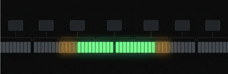
Sqrt-decomposition is somewhere between these two: low-cost, not-too-complicated preprocessing and implementation. In this approach, the data array is split into sqrt(N) = B blocks (and B elements in each block); each block computes its own independent aggregate. And so, when you need to update the element, you add it to the required block and recalculate the aggregate for that block; the complexity of this operation varies from O(1) for operations like sum/multiplication to O(B) and O(B log B) for more complex operations like finding a minimum/maximum or sorting a block. Next, when you are querying the aggregate over the l to r segment, you would use these 3 steps:

• Linearly calculate the aggregate for the partial block located on the left edge, where l falls in the middle of a block.
• Walk through the blocks that are fully located inside the l..rsegment.
• Linearly calculate the aggregate for the partial block located on the right edge, where r falls in the middle of a block.

In the above picture, you can see the full and partial blocks you need to process to compute the aggregate for the range from l to r.

Since all of these parts take at most O(B) time to compute, a range query takes O(B), which is O(sqrt(N)). The update operation has similar complexity because when you modify a single element, you only need to recalculate the aggregate for the block that contains that element.

ClickHouse MergeTree

Before comparing this with sqrt-decomposition, it is worth looking at how ClickHouse stores data in MergeTree tables. Inserted data is organized into immutable parts, which are later merged in the background. Within each such part, rows are grouped into index_granularity-sized granules (by default, index_granularity is 8192). Instead of storing an index entry for every row, ClickHouse stores one sparse-index entry, or mark, per granule. This is much cheaper: the index stays small, while each mark is still enough to point ClickHouse to the right place in the column files.

The analogy with sqrt-decomposition is easiest to see at the granule level. The “block” in the sqrt-decomposition model corresponds roughly to a granule in MergeTree. However, you cannot say that the mark is a precomputed aggregate, as in the square-root summary. It is the primary-key value at the granule boundary, together with an offset. This is still enough because MergeTree data is sorted by the primary key: boundary values alone tell ClickHouse which granules may fall within a query’s range.

When rows are sorted, the boundaries of adjacent granules indicate ranges of values. Therefore, when a query limits results by the sort key, ClickHouse uses the sparse index to determine which granules may contain matching rows, and reads only those granules, skipping the rest.

Overall, ClickHouse provides benefits similar to those of sqrt-decomposition. Both techniques allow large portions of data to be skipped, but they do it in slightly different ways. In sqrt-decomposition, each block usually has a precomputed summary. In MergeTree, the mark is closer to a boundary marker over sorted data, with an offset into the column files.

The closest similarity appears at the edges of a range query. Since ClickHouse reads data at the granule level, it still must read the entire granule and discard rows that fall outside the requested range. In the worst case, a primary-key range query may read up to 2 * index_granularity extra rows, coming from one partially covered granule on each side of the range, which is the same situation as with partial blocks in sqrt-decomposition.

In both cases, most of the range is cheap to handle, but the edges may still cost almost a full block. The sparse index helps with filters on the sort key; for other columns, ClickHouse uses skip indexes. Skip indexes can hold a min/max value for a column per granule (or group of granules). This is close to the original sqrt-decomposition idea: maintain a compact summary of the block to determine whether it can be ignored.

For example, for a one-billion-row table with the default 8192-row granule size, this gives about 122,000 marks, which is small enough that the sparse index usually stays in memory. ClickHouse may only need to scan the sparse index and read a small number of consecutive granules if the filter matches a narrow range of the sort key. If the filter is on another column and there is no helpful skip index, the sparse index cannot help nearly as much, and ClickHouse may have to scan much more data.

Prometheus TSDB

Prometheus has a similar block-shaped read path, although its blocks are produced through a different lifecycle than in the simple sqrt-decomposition model. Incoming samples are first written into an in-memory head block, where samples for each series are stored in chunks of around 120 samples, following the chunk size used in the Gorilla work at Facebook for delta-of-delta compression. The head is flushed later to the disk, but here is what makes this engine different from others: instead of having a block size defined as a certain amount of records/bytes/etc, it defines a block as a 2-hour time range of data, which makes sense if your range requests are primarily time-focused. When the head is added to the disk, it becomes an immutable block that contains an index, compressed chunks, and a meta.json file with the minimum and maximum time covered by that block, which Prometheus can use to avoid blocks that are outside the query’s time range.

The compactor then merges blocks into larger time ranges: three 2-hour blocks become a 6-hour block, three 6-hour blocks become an 18-hour block, then a 54-hour block, and so on. Prometheus, similar to sqrt-decomposition, works with blocks. The difference is that older blocks are also rewritten into larger ones to avoid accumulating too many small files, which is closer to an LSM-style design.

InfluxDB TSM and IOx

Let's start with the earlier version of InfluxDB and see how it stores data. When it receives data, it first splits it into time-based blocks corresponding to a shard. With an indefinite retention policy, this usually means one shard per week. The data inside each shard is stored in TSM files, which are sorted, compressed, immutable, and merged through compactions.

The main point you can draw an analogy to with sqrt-decomposition is how the data is stored in these TSM files. Their indexes store the offset, the block length, and the minimum/maximum timestamps of the data inside. So, thanks to these timestamps, during the request, you can only scan those index entries and read only the blocks that may still contain matching data.

Later, the InfluxDB team replaced the original approach with the IOx storage engine. In the new implementation, the read path goes through the catalog to find the relevant files (Parquet) that store the required information (such as min/max time) for rows and columns of the database, which helps locate the requested query range. So, the details were changed, but the pattern stayed close to the old one and to the sqrt-decomposition approach.

The common shape, made explicit

The table below matches the square-root decomposition model with the closest mechanism in ClickHouse, Prometheus, and InfluxDB.

| square-root decomposition | ClickHouse MergeTree | Prometheus TSDB | InfluxDB (TSM and IOx) |
|---|---|---|---|
| Block | Granule (8192 rows) | Chunk (about 120 samples), then 2h block | TSM block, or Parquet row group |
| Block size B |
| samples per chunk, block duration | block size, shard or partition duration |
| Per-block summary | Sparse mark (boundary value, relies on sort order); minmax skip index for a true aggregate | meta.json min and max time | TSM index min/max time, or Parquet column-chunk statistics |
| Whole-block skip | Granule pruning via marks | Block selection via meta.json | Shard and block pruning, or partition pruning via the catalog |
| Scan the edge blocks | Up to | Decode partial chunks at the edges | Decode partial blocks at the edges |
| Coarsening by compaction | parts merged into larger parts | 2h merged into 6h, then 18h, 54h | shard, then TSM levels 1 to 4 |
| Cheap point update | append to a new part | append to a head chunk | append to WAL and cache |

As you can see, the same idea shows up differently in each system, and despite different terminology, these systems all have similar block-based read paths. This is a natural approach for append-heavy data, range queries, and a constant need to avoid unnecessary reads.

Blocks instead of trees

Let's compare the sqrt-decomposition approach with trees. Using a segment tree or a balanced search tree with O(log N) seems like a better choice than sqrt-decomposition with O(sqrt N), if you compare only by asymptotic running time. From that comparison alone, you can assume that trees are the best choice all the time, and that sqrt-decomposition is just an easier data structure to start with.

But this assumption fails to consider the fact that the comparison is usually made in the classic case where data changes frequently and randomly, with many updates to existing data. In our case, this is not true; the data in databases mostly appears at the end of the whole queue, and old data is rarely modified in place. So trees are not helpful in such situations, and they can even bring random seeks, pointer chasing, and rebalancing work across levels.

For data storage systems using the sqrt-decomposition approach, when new data arrives, it is filled into the block at the end of the existing queue. Then the system calculates min/max timestamps, and uses these values to determine when the block needs to be read, depending on the time range in the request. Because appending to the current block is cheap due to a different memory access pattern and the expensive case of recomputing old blocks is rare, using sqrt-decomposition is an advantage in this case.

Where the model breaks, and why that is the useful part

While the sqrt-decomposition model is good to start with and explain how the algorithm works and what the main advantage of this approach is, in reality, this model breaks down multiple times. This is expected: production systems with specific use cases, constraints, and costs differ from a well-polished theoretical problem. However, these differences shouldn’t be perceived as disadvantages, as they are aimed at optimizing the system, and understanding them is essential for using them efficiently. Let’s elaborate on these points.

The first thing to understand is that systems don’t choose B = sqrt(N) as the block size, and the reason is simple: the data size doesn’t change in the classic problem, while it constantly grows in production systems. Making the block size dynamic and increasing it would degrade the system over time and create an anti-pattern: the longer the system exists, the longer it takes to pull the most recent data. Meanwhile, in reality, you usually want the opposite: an easy way to access the most recent data (last day/week/month), while getting data from the last year or a few years ago can take longer and is not a concern. Instead, systems choose a fixed B, which provides block size and processing stability, and use compression for older blocks of data to save memory for queries that are rarely called.

Another reason sqrt(N) is a bad idea is the assumption that both block update and result accumulation operations have an O(1) complexity, which might also be incorrect. This is not even true for some classic sqrt-decomposition problems, where calculating a result from a block can take O(log N) if you have to search in sorted data. Also, the constant time complexity in both cases doesn’t mean the same time, and modifying the block size might improve the actual processing time if the complexity looks “worse”. Another consideration is that, in practice, building the block requires running a compression or sealing algorithm to represent the information in a way that makes query calculations efficient. That’s why real systems use custom block sizes depending on their compression algorithms: 8192 rows, 120 samples, or even time-range-based, such as two hours.

The second point is that decomposition, in fact, is not one-dimensional, but rather two-dimensional. For most databases, queries don’t just require requesting data for a specific period of time. Usually, they have to filter by labels, such as request status, caller ID, or latency  (e.g., http_requests{service="checkout", status="500"}).  These labels could be different, such as the request status, caller ID, latency, etc. This involves adding one more axis: in addition to the time axis, the labels axis needs to be added, and it is managed by another mechanism, such as an inverted index with postings lists and roaring bitmaps in Prometheus or TSI in InfluxDB. That means sqrt-decomposition explains the first dimension, but the second dimension is another level of abstraction with its own latency and limitations, and is not as simple as the initial concept of sqrt-decomposition is. As a result, the range query will depend on the intersection of two completely different concepts and data structures.

The third difference is that you can’t and don’t need to do an in-place update in O(1). The concept of sqrt-decomposition assumes that updates will be distributed randomly across the range and is good at optimizing the worst case, but, in fact, most time-series databases just need to append data to the end of the structure (such as real-time metrics and logs), with some tolerance to data that arrived late due to network latency or outages. Also, these appends mostly happen before the head block is built & sealed. However, an additional cost of the summary is still present in these databases, but it is related to the block compaction performed by systems in the background. This also changes the nature of how these databases accept appends to blocks that are already sealed/compressed/compacted: Influx DB allows that and does a multi-level compaction to merge data into a single block if there are past appends, ClickHouse accepts them easily but makes the cost of compaction expensive later, meanwhile Prometheus declines appends that are not part of the head block completely.

How to use this insight

This insight not only explains how things work in general but also helps developers utilize these databases more efficiently. Here are key takeaways from understanding that block decomposition lies behind these solutions.

Block size is the knob. All three databases take block size as a knob, which trades off 4 properties against each other: pruning accuracy vs scanning throughput (large blocks allow more scans while smaller blocks mean more granularity) and in-memory index size vs compression (large blocks are easier to compress while smaller blocks allow more details to be described). Depending on the nature of data & queries, an efficient database configuration may vary, and understanding block decomposition principles helps understand these trade-offs.

Single reads are slow. As all engines compress data to blocks, they cannot read a chunk of data smaller than a block size, even when you need to read a single row. This thing cannot be tuned in these databases, and understanding this will help an engineer decide to move to another data storage if this type of query is common in their use case.

Range query performance. Understanding how the data structure works shows that the performance of a range query is strictly tied to the data structure that is used behind it in a database. Knowing how the query is executed can help evaluate the performance of the range query and write your code most efficiently. This insight also allows an engineer to design additional indexes and data structures correspondingly: they don’t have to think about a different approach, but can follow the same structure as their database.

This insight doesn’t change our understanding of ClickHouse merges and Prometheus compaction, and it shouldn’t. The main takeaway from this material is that principles that are true for sqrt-decomposition (partition by query dimension, precompute the result for each block, and use them when executing a range query) are valid for most time-series databases. Use this wisely when designing your systems.

References

• ClickHouse Documentation: A practical introduction to primary indexes
• ClickHouse Documentation: MergeTree Engine
• Prometheus Documentation: Storage
• G. Vernekar: Prometheus TSDB blog series
• T. Pelkonen et al.: Gorilla - A Fast, Scalable, In-Memory Time Series Database
• P. Dix: The New InfluxDB Storage Engine - Time Structured Merge Tree
• InfluxDB Documentation: In-memory indexing and the TSM
• InfluxData: Introducing InfluxDB 3.0
• Apache Parquet: Documentation
• P. O'Neil et al.: The Log-Structured Merge-Tree (LSM-Tree)
• A. Laaksonen: Guide to Competitive Programming
• CP-Algorithms: Square-root decomposition