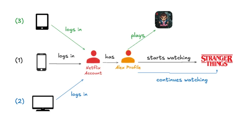
How and Why Netflix Built a Real-Time Distributed Graph: Part 3 — Querying the graph with gRPC execution APIAuthors: Nilesh Mishra and Ajit KotiThis is the third entry of a multi-part blog series describing how we built a Real-Time Distributed Graph (RDG). In Part 1, we discussed the motivation for creating the RDG and the architecture of the data processing pipeline that populates it. In Part 2, we discussed how we designed the storage layer to handle billions of nodes and edges while maintaining single-digit-millisecond latency. In Part 3, we will explore how we designed a fast, flexible serving layer to efficiently query the graph.IntroductionIn Part 1 of this series, we described why Netflix needed a Real-Time Distributed Graph (RDG) and how we used Apache Flink to build an ingestion and processing pipeline that turns streaming events into graph primitives. In Part 2, we explored how we designed a storage layer capable of handling billions of nodes and edges while still delivering single-digit-millisecond latency.In this post, we focus on the next challenge: querying the graph efficiently to power real-time insights for our internal partners. All of the work on ingestion and storage only matters if we can actually ask complex questions and get answers back quickly. As we optimized for lower latency, we found that the serving layer posed its own set of challenges, distinct from those of ingestion and storage. How do we turn a constantly evolving, billion-edge graph into sub-100ms responses across a wide variety of workloads? This is the problem we tackle in this post.The Real World NeedsAs we integrated the RDG into Netflix’s ecosystem, we realized that “querying the graph” is not a one-size-fits-all operation. We needed to handle a wide range of access patterns: from high-volume security lookups to deep, exploratory personalization traces.Let’s revisit our example from Part 1 and expand on it slightly. In the earlier posts, we focused on accounts, devices and content. In practice, the graph is richer: each account has multiple profiles.A member journey often looks like this:Alex logs in to their Netflix profile on a smartphone and starts watching Stranger Things.They later switch to a smart TV in the living room to continue the episode.The next morning, they use a tablet to play the game Stranger Things: 1984.In the RDG, this journey creates the following graph structure:Graph queries vary along two axes: how wide they fan out at each hop, and how deep they chain across hops. To see this range, let’s look at two scenarios from opposite ends:1. Shallow and wide: “Which devices has this account used?”Consider a “shallow, wide” query: “Which devices has this account used to stream in the last 30 days?”Using the graph structure above, this translates to:Starting Point: A specific Account Node.Hop 1 Edge Traversed: The streamed_from edge.Hop 1 Destination: Device Nodes.While this is only a “single hop,” it presents a significant scaling challenge. For a highly active account, the fan-out can be massive. The query layer must fetch hundreds of streamed_from edges, apply temporal filters on each edge’s last_watch_timestamp property to capture only those within the last 30 days, and aggregate the results, all while maintaining sub-100ms latency.2. Deep & Narrow: What has this profile watched?Consider a scenario where personalization teams need to understand a member’s viewing journey. They might ask: “For Account X, show me the Stranger Things viewing history across all profiles: which profiles watched it, what they watched, and when”.This path unfolds as follows:Starting Point: A specific Account Node.Hop 1 Edge Traversed: has_profileHop 1 Destination: Profile NodesHop 2 Edge Traversed: started_watching (filtered for title_name = “Stranger Things”)Hop 2 Destination: Content NodesThe core challenge in this scenario is sequential dependency: we cannot fetch a profile’s viewing history until Hop 1 has identified which profiles exist. In a distributed environment, the client has to wait for Hop 1 to finish before sending Hop 2. If each hop takes 10ms of network time, that’s 20ms of overhead before we’ve processed a single byte. To hit our sub-100ms goal, we needed a way to package this multi-step logic into a single request.This example is a 2-hop traversal, but queries can chain 3–4 hops across different entity types, and the latency penalty of sequential execution only grows with depth.Balancing Depth and BreadthThese two scenarios pull the system in opposite directions. Shallow-wide queries stress I/O throughput: can we handle massive fan-out without slowing down? Deep-narrow queries stress execution efficiency: can we chain multiple hops without the network overhead adding up? Supporting both on the same system is what shaped the design that follows.Design Constraints and Key ChoicesThe two scenarios above sit at opposite ends of the spectrum, but they are not unusual. In practice, the RDG serves tens of thousands of queries per second, each potentially different, all needing sub-100ms responses while the underlying graph continues to grow. Scale, latency, query diversity, and the need for extensibility pulled the design in different directions at once, and every choice came with a trade-off we had to live with.Why breadth-first, not depth-first? The most intuitive way to traverse a graph is depth-first: pick a path, follow it to the end, backtrack, try another path. But in a distributed system where every hop is a network call, depth-first can lead to high latency. If Account X has 5 profiles and each profile has watched hundreds of titles, depth-first would trace all of one profile’s watched titles before moving to the next, missing the opportunity to batch lookups across profiles. Breadth-first flips this by working one level at a time across all nodes, rather than one path at a time through each node. We fetch all profiles for the account at once, then fetch the started_watching edges for all profiles, and finally fetch content details for all matching titles. Three rounds of parallel calls instead of sequential chains. With breadth-first, there is a clear trade-off in memory, because we hold each level of the graph in memory at once, so the cost scales with how wide a level fans out rather than how deep the query goes. We keep this comfortable by bounding each hop with the per-edge-type limits described in Step 5 below, so even a high fan-out level stays a manageable frontier. We’ll walk through how this works, level by level, in Step 3 below.Why async-first, not thread-per-request? Latency in the RDG is dominated by I/O, reading from the storage layer, calling enrichment services, and waiting on caches. A traditional thread-per-request model would pin a thread to each in-flight query, and most of the time, the thread would be idle, waiting for a network response. With thousands of concurrent queries, we’d need thousands of threads, most of which would be doing nothing. Instead, we decided to build the entire execution pipeline around asynchronous composition. A small set of dedicated thread pools (16–24 threads total) handles thousands of concurrent requests because no thread ever blocks on I/O. While a storage call is in flight, the thread continues with other work and picks up the result when it arrives. This is the foundational design decision on which everything else rests. We’ll see this in action in Step 4 below, where we cover parallel execution.Why cache selectively, not everything? Not all data in the graph changes at the same rate. Some properties, such as account plan type and content metadata, are relatively stable: they change on the order of hours or days. Edges like who watched what and when change constantly. For stable data that many queries touch, we use a distributed cache (EVCache) with TTLs tuned to data volatility. Getting the caching strategy right took iteration. We started by caching aggressively and measured the impact: tracking hit rates, monitoring stale-data incidents, and adjusting TTLs based on how quickly different node types actually changed in production. The result: 70–80% hit rates on node lookups, achieved by narrowing the cache to nodes that are both frequently accessed and slow to change, while skipping data that would expire before the TTL ran out. Step 6 below covers how this works in practice.Why opt-in enrichments, not automatic? Clients know what they need. A query checking account relationships doesn’t care about title artwork; a personalization service building a viewing timeline does. Rather than fetching metadata from external services by default and penalizing every query, we make enrichments opt-in: clients specify exactly which external data they want per request. Also, enrichment is fail-open: if a service is slow or unavailable, we return the graph data without it.Why eventual consistency, not strong? Most of our queries ask “What has this member done recently?”, not “What happened in the last millisecond?” By defaulting to eventual consistency, we read from the nearest replica and avoid coordination overhead. While the RDG is used to power in-the-moment experiences, it is not set up as the source of truth for the data it holds.Architecture OverviewThe above choices lead to the following three-layer architecture:The Graph Query Service is the entry point. It accepts gRPC requests, validates the traversal specification, and hands it to the query execution engine. The execution engine orchestrates breadth-first traversal: expanding one level at a time, applying filters and limits at each hop, and composing all I/O asynchronously.The Storage Abstraction Layer sits between the execution engine and the underlying KVDAL storage. It provides a clean interface for node lookups and edge retrieval, handles streaming for large adjacency lists, and manages node caching (EVCache).The Enrichment Layer fetches additional metadata from external Netflix services on demand. It batches requests, runs them in parallel with graph data assembly, and degrades gracefully when an enrichment source is unavailable.When a client sends a query, the request flows through these layers in sequence: the Query Service parses the request into an execution plan, the execution engine walks the graph level by level through the Storage Abstraction Layer, and if enrichments are requested, the Enrichment Layer fetches and merges external data before the response is serialized back to the client.Now, with that mental model in place, let’s follow a query through this system and see how these choices play out in practice.Executing Queries Efficiently: Following a Query’s JourneyTo see how the RDG query layer works in practice, let’s follow a single query end-to-end and focus on one question: how do we make every step fast?We’ll reuse the deep-narrow example from above:For Account X, show me the Stranger Things viewing history across all profiles: which profiles watched it, what they watched, and when.In graph terms, this becomes a 2‑hop traversal:Account X → has_profile → ProfilesProfiles → started_watching → Content (filtered for “Stranger Things”)We’ll walk through how this query moves through the layers we described above:Reading and interpreting the requestReading from storage efficientlyExecuting traversal with breadth‑first levelsRunning many operations in parallel, but safelyFiltering smartly to keep only what mattersMaking repeat queries faster with cachingBy the end, we’ll see how a 2-hop query like our Stranger Things example, with streaming, filtering, and parallel execution, can complete in under 100ms.Step 1: Reading the Request: Deciding What the Query Really WantsEvery query starts as a gRPC request. Before we touch storage or walk a single edge, the engine needs to understand what the caller actually wants.For our running example below:For Account X, show me the Stranger Things viewing history across all profilesThe engine creates a traversal plan with a set of levers: how many hops, how many edges per hop, how much history to consider, and whether to favor recent activity.We resolve these upfront by merging a hierarchy of filters and limits, from application-level defaults down to per-edge-type overrides, into a concrete execution plan. By the time we read from storage, every hop has clear rules. We’ll see how this hierarchy works in detail in Step 5, but the key insight is simple: interpreting the request up front prevents over-fetching from the downstream storage layer.Step 2: Reading from Storage: Direct Lookups and Streaming Fan‑OutOnce we’ve parsed the request and decided what the query should do, the next step is to actually touch the graph. For our running example:For Account X, show me the Stranger Things viewing history across all profiles…The first concrete question the engine has to answer is very simple:Which profiles does Account X have?Under the covers, that really means: how do we find all relevant edges for Account X without scanning the entire graph every time?Finding Edges Fast with Adjacency ListsIf we stored every edge in one massive table, the naive approach would be to scan for rows where source = Account X. Even with indexing, doing that across billions of edges for every request would be slow.Instead, we organize edges as adjacency lists. For each node, we keep a compact list of “who it’s connected to” by edge type. For Account X, a simplified view might look like:Account_X: has_profile → [Profile_Alex, Profile_Kids, …,]Now “get all profiles for Account X” is no longer a global search; it’s a direct lookup into Account X’s stored adjacency. The storage layer can usually pull that list back in a few milliseconds because it’s reading a small, well‑indexed slice of data instead of hunting through everything.For our query, the first hop is quick: Account X has just two profiles. The engine fetches those edges with has_profile and moves on. For more information on Storage, refer to our previous post.When One Node Has A Lot of NeighborsThe first hop was small, but the second is where things get interesting. Each profile can have a large number of started_watchingedges. Loading the entire adjacency list at once would spike latency and memory usage.To avoid this, we treat adjacency lists as streams rather than blobs.When the engine requests Profile_Alex’s started_watching edges, the storage layer streams them in batches of 100. As each batch arrives, we apply filters (e.g., “last 30 days”) and decide whether to continue.If we’ve collected enough edges to satisfy the query’s limits ( max_edge_cnt, lookback window, etc.), we stop reading. Otherwise, we pull the next batch.In our Stranger Things example:Storage streams the started_watching adjacency for Profile_Alex.There are about 500 edges total: months of viewing historyAs each batch arrives, we filter for Stranger Things and drop anything older than 30 days.After a few batches, we’ve found what we need: a handful of Stranger Things sessions.We never materialize more data than needed. Filtering happens at the source.Why This Matters LaterThese two choices, the adjacency‑list lookups and streaming fan‑out, enable everything that follows:Small fan‑outs (like Account → Profiles) yield predictable, low‑millisecond lookups.Large fan‑outs (like Profile → Content) stay efficient by reading only what’s needed.Traversal logic treats “neighbors of this node” as a cheap, bounded operation.By Step 3, we’re working with concise frontiers like “Profile_Alex and Profile_Kids,” ready for the next hop into their viewing histories.Step 3: Traversal Execution: Walking the Graph Level by LevelWe’ve completed the first hop. From Account X, we pulled the has_profile edges and found two profiles: Profile_Alex and Profile_Kids.But we’re not done. The query was:For Account X, show me the Stranger Things viewing history across all profiles: which profiles watched it, what they watched, and whenSo we still need to fetch each profile’s history and filter it down to Stranger Things sessions. As we covered in our design choices, we use breadth-first traversal: expanding all nodes at the current level in parallel before moving to the next.Querying, Level by LevelLet’s walk through the Stranger Things query level by level.Level 1: Account → ProfilesStarting at Account X, the engine pulls has_profile edges, discovering two profiles:Profile_Alex, Profile_KidsThese become the frontier for Level 2, a single small lookup that takes a few milliseconds.Level 2: Profiles → Content (Stranger Things)From those two profiles, we fetch started_watchingedges and filter for Stranger Things. Instead of exhausting Profile_Alex’s entire viewing history before touching Profile_Kids, we treat this as one logical step:For each profile, fetch started_watching edges in parallel.Filter for title_name = “Stranger Things” as edges stream in.Each profile might have hundreds of content edges, but filtering at the source keeps the result set small.We discover that Profile_Alex watched Season 1 and Season 2, while Profile_Kids watched Season 4. Level 2 turns “2 profiles” into “a handful of Stranger Things sessions” in roughly one storage round trip.The traversal completes: two levels, two frontiers.Why This Matters for LatencyWe parallelize within each phase, then regroup. This provides:Predictable resource usage: known requests per levelMaximum parallelism: all frontier nodes processed togetherFar fewer round trips: one per level, not per pathFor a 2-hop query: two rounds of parallel lookups instead of hundreds of sequential ones. That’s why our Stranger Things query completes in under 100ms.Step 4: Parallel Execution: Doing Many Things at Once, SafelyBreadth-first traversal enables parallel work at each level, which is the key to low latency.At Level 2 of our Stranger Things query, we fetch started_watching edges for each profile. With two profiles, this is trivial, but in production queries fan out across many profiles, each with hundreds of edges to stream and filter. So do we process them sequentially or in parallel? Sequential means waiting for each profile before starting the next, and the delays stack up. Parallel finishes in the time of the single slowest profile, but hundreds of queries doing this at once could overwhelm storage with unbounded concurrency.The goal: parallel speed without unbounded chaos.A Kitchen, Not a Single QueueWe structured the query engine like a professional kitchen, with specialized stations for appetizers, mains, and desserts, each with its own capacity. If one station is slammed, the others keep flowing. In practice, that means dedicated thread pools for different work types: fetching nodes, reading adjacency lists, and performing enrichments. When the Stranger Things query reaches Level 2, calls route to the adjacency-list pool, where 8 workers stream and filter each profile’s edges in parallel.Knowing When to Back OffThread pools give us local control, but we also need a global view of total capacity, so we use adaptive concurrency limiting. When things are healthy, we raise the limit gradually (100 in-flight, then 101, 102, and so on); when timeouts or errors spike, we back off by a larger step (say, 100 down to 70). Combined with per-pool limits, the engine constantly tunes parallelism, fanning out within each level while staying inside safe storage and network limits.Fetching Extra Metadata Along the WayIf the client opted into enrichments (say, maturity ratings for the matched content), the Enrichment Layer fetches them in parallel on its own thread pool and merges them into the response. Enrichment is fail-open: a slow or unavailable source never blocks the query, and we just return the graph data without it.​​Step 5: Smart Filtering: Keeping Only What MattersWe’ve traversed from Account X to profiles, then to their viewing histories. But raw edges aren’t what our partners need. They care about recent, relevant activity, not every started_watching edge accumulated over the years. This is where filtering decides which parts of the story make the final cut.From “All Activity” to “The Last 30 Days”Go back to the original question:For Account X, show me the Stranger Things viewing history across all profiles: which profiles watched it, what they watched, and when.The phrase “viewing history” is deceptively simple. Under the hood, it means we need to:Ignore older viewing activity, even if it exists in the graphAvoid pulling more edges than we actually needLet different teams choose their version of “recent enough.”We handle this with a filtering hierarchy. The system starts with conservative defaults (e.g., 100-day lookback, 300 edges per hop), and requests can override them globally, per-hop, or down to specific edge types. In our query, the 100-day default applies broadly, but the caller sets 30 days for started_watching edges, and the narrower rule wins. Older sessions are discarded. The same engine can just as easily provide a tight recent window on one edge type and full history on another, all in a single query.Choosing Which Edges to Keep: LATEST vs ANYSometimes there are still more edges than we want to return after time filtering. If Profile_Alex watched the same episode several times last month, pausing and resuming, we don’t want to send all those edges back. So we offer two selection modes.LATEST sorts edges by timestamp and keeps the newest ones up to the limit, ideal for “what has this profile watched recently?” where teams want the current state, not every play event. ANY grabs whichever edges it encounters first, no sorting, which is faster and fine for “has this profile ever watched Stranger Things?” where timing doesn’t matter. Teams default to LATEST and switch specific edge types to ANY when “any proof” is enough.Bringing It Back to Our StorySo what happens for our running query?We start with all the started_watching edges for each profile. The time filter narrows this to 30 days. Edge-count limits prevent response flooding. LATEST mode selects the most recent viewing session per title. The result: a concise answer distilled from a verbose history:Profiles that watched Stranger Things in the last month.Which seasons and episodes they watched.The most recent session for each, tying it all together.This filtering turns raw history into a focused answer.Step 6: Making It Even Faster: Caching the Things We Keep SeeingBy now, we’ve walked the full path of our query: we’ve traversed from account to profiles, filtered viewing history by time, and focused on Stranger Things sessions.Despite our optimizations, each storage call still costs a network round-trip. When the same nodes appear across thousands of queries per minute, those redundant calls add up: both in infrastructure cost and in tail latency at scale.The key question: what can we avoid repeating?The Things That Don’t Change Every SecondLook back at the entities in our Stranger Things journey:The Account node (plan type, region, etc.)The Profile nodes (“Alex”, “Kids”, whether it’s a kids profile)The Content nodes (Stranger Things seasons and episodes)These rarely change. Profiles don’t flip between “kids” and “non-kids” every minute. Title metadata is stable.To improve efficiency, we keep a distributed cache of hot nodes (accounts, profiles, content) that are likely to reappear. When the same entity appears again, we answer “What is this node?” from memory, skipping storage.Result: for high-traffic entities, we eliminate storage calls and noticeably reduce infrastructure cost and tail latency at scale.A Quick Replay of Our Query With Caching Turned OnThe first time the Stranger Things query runs for Account X, the cache is cold, so we pay the full cost: we fetch the account and its profiles, then the started_watching edges and matching content nodes, caching each node as we go. Minutes later, a different query arrives:Show me everything Account X’s profiles have watched in the last 7 days, and flag anything rated TV-MA on the kids profile.This time, many of those nodes are already in the distributed cache. Storage still handles the adjacency lists and edges, but node lookups are lighter and latency drops. At scale, that reuse gives us comfortable headroom for traffic spikes.Not Everything Deserves a Spot in CacheWe can’t cache everything. The RDG prunes old activity after a set retention window, so caching a node that’s about to be deleted is wasteful.To avoid polluting the cache, we consider:The node’s last activity timestampThe graph’s retention period (e.g., 100 days)The cache TTL (e.g., 30 days)If a node was last active 99 days ago, it expires from the graph in a day, so a 30-day TTL makes no sense, and we skip it. We reserve cache space for active nodes like Account X. This “smart TTL” policy keeps the cache focused on live stories rather than archival ones, so repeat queries for the same part of the graph return faster.Caching is integrated into the journey, not an afterthought. The engine reuses knowledge from previous queries, so repeated traversals over the same part of the graph keep getting cheaperThe PayoffThe serving layer sits in front of 8 billion nodes and 150 billion edges, serving mixed workloads, all of which need to feel interactive. Single-hop queries return at a P50 of 15–30ms with P99 under 100ms. Even 3-hop traversals, the kind that chain across accounts, profiles, and content, come back at P99 between 100–150ms. Breadth-first execution and parallelism within each level keep these numbers stable even as fan-out grows.The async-first design is what enables the throughput. Thousands of concurrent requests flow through just 16–24 threads spread across dedicated pools because no thread ever blocks on I/O. When load spikes, our concurrency limiter lets work queue briefly: slowly increasing capacity when things are healthy, backing off aggressively when they’re notCaching has the most visible impact on day-to-day efficiency. Popular entities like accounts, profiles, and content achieve 70–80% cache hit rates, resulting in roughly 3–4x fewer storage calls on common query paths. Smart TTLs keep the cache focused on active data, avoiding wasted memory on nodes that are near the end of their graph retention window.These properties, together, make multi-hop graph queries over billions of entities feel, at query time, much closer to in-memory lookups than to remote calls.What We Learned Along the WayThe biggest surprise wasn’t any single optimization: it was how much async composition changed the economics of our system. We expected it to help latency; we didn’t expect it to slash infrastructure cost. A serving layer that would have needed hundreds of threads per instance runs comfortably on 16–24, because no thread ever blocks on I/O. The tradeoff is debuggability: async stack traces are hard to read, and exceptions can get lost in future chains. We compensated with per-stage metrics, measuring each request at validation, storage, enrichment, and end-to-end, so when something is slow, we know exactly which stage to blame.Caching took longer to get right than expected. Our first instinct was to cache everything in EVCache and let TTLs handle freshness, but that wastes memory on nodes about to expire from the graph anyway. The breakthrough was matching TTLs to data volatility: stable node properties get long TTLs, while nodes near the end of their retention window aren’t cached at all. The 70–80% hit rate we see today came from being selective, not aggressive.The filtering hierarchy was born out of frustration. Early on, every new use case meant a code change: one team wanted a 7-day lookback, another 90 days, a third different limits at different depths. Instead of bespoke logic per team, we built a layered override system: application defaults, global overrides, per-depth limits, and per-edge-type limits. It took real effort, but it eliminated an entire class of feature requests and teams now tune their own queries without touching our code.Closing: Principles for Distributed SystemsThe lessons above are specific to the RDG, but the underlying principles apply to any distributed system built around I/O-heavy, fan-out workloads.Think in terms of frontiers, not features. Design your APIs so callers describe what frontier to explore, then let the system decide how to walk it efficiently.Filter early, not late. Every byte you fetch but don’t need is wasted I/O. Push filters and limits as close to the storage layer as possible: discard irrelevant data at each stage rather than fetching everything and trimming at the end.Parallelize deliberately, not by default. Unbounded concurrency feels fast until it overwhelms the systems you depend on. Set explicit limits, monitor them, and adjust dynamically: treat concurrency as a dial, not a switch.Treat caching as a first‑class design choice, not an afterthought. Decide what is worth remembering, for how long, and what should be allowed to fade out of memory. Match TTLs to data volatility, and don’t cache what’s about to expire.—Thanks for reading Part 3 of the RDG blog series. For us, getting these details right is what turns a constantly changing, billion-edge graph into something that, at query time, feels like a responsive, in-memory data structure.How and Why Netflix Built a Real-Time Distributed Graph: Part 3 — Querying the graph with gRPC… was originally published in Netflix TechBlog on Medium, where people are continuing the conversation by highlighting and responding to this story.