Tabular LLMs: An Introduction to the Foundation Models That Predict Your Spreadsheet

There is a fairly new class of model for tables: pretrained transformers that predict on any spreadsheet zero-shot, loosely called “tabular LLMs”. On the TabArena leaderboard, every single-model entry above the best tuned, ensembled GBDT configuration is one of them; the only entries above it that aren’t are AutoGluon’s 4-hour ensemble pipelines. That inverts the default answer of the last decade, which was to fit a tuned gradient-boosted tree. Leaderboards have been wrong before, in ways that only show up when an outsider re-runs them (that was my experience with time-series models), so before believing this one I audited it. I recomputed the board’s scoring from its published artefacts, took TabICLv2, the strongest model on it with unrestricted open weights, and re-ran it from scratch on hardware I controlled.

My independent run covered all 51 datasets on the benchmark’s official Lite protocol (one train/test split per dataset, the same split indices the leaderboard uses) on a single AWS A10G. Scored against the official artefact rows on those identical splits, my TabICLv2 lands at Elo 1559 against the official 1575, adjacent ranks and well inside the ±60–86 bootstrap intervals. Per task, 16 of the 51 metric values came back identical to four decimal places, the median relative difference was 0.08%, and the worst dataset differed by 3.5%, the size of gap you’d expect from GPU nondeterminism rather than a methodology difference. The whole sweep, environment setup included, fitted in a 2.1-hour GPU session that cost just over $2.

What a tabular foundation model is

A tabular foundation model is a single pretrained model that predicts on any table, zero-shot. You hand it the rows whose labels you know as context, the way you would paste worked examples into an LLM prompt, and it predicts the labels of the held-out rows in one forward pass. Nothing gradient-trains on your data and there is no hyperparameter search; the step every other tabular method calls “training” becomes inference. The literature calls this in-context learning, and the TabPFN papers established that it works for tables.

It behaves like a learned k-nearest-neighbours: to label a held-out row, the model attends over the rows whose labels it can see and reads off an answer weighted by how similar they are. The difference from ordinary k-NN is that the similarity, and the way neighbours are combined, come from pretraining rather than being fixed in advance.

The family has grown fast since: TabPFN’s successors (Prior Labs), TabICL and TabICLv2 (Inria’s SODA team), TabDPT (Layer 6), and, two weeks before this post, Google Research’s TabFM. All of them appear in the standings below.

The “LLM” in “tabular LLM” is loose. These models are transformers, but they do not model language, and they differ from a text LLM in every ingredient. A text LLM’s token is a word-piece from a fixed vocabulary; a tabular model’s raw material is the cells, columns, and rows of a table, numbers and categories with no fixed vocabulary at all, since your table’s columns have never been seen before and the model has to cope anyway. A text LLM pretrains on internet text with next-token prediction; a tabular foundation model pretrains on millions of small synthetic tables generated by random structural causal models (random cause-and-effect graphs wired up to emit plausible fake datasets), and its objective is to predict the held-out cells and labels of those tables. Pretraining instils a general procedure for reading a fresh table and inferring how its features relate to its target, rather than knowledge about the world. One consequence is size. Tables carry less surface complexity than language, so tens of millions of parameters are enough: TabICLv2 is about 28M, against t0-alpha’s 102M and a text LLM’s billions.

The contrast with the time-series foundation models from the t0 post comes down to order. A time series has one: t0, Chronos, and TimesFM apply causal attention along time, only ever looking at the past, and forecasting means continuing the sequence beyond its end. A table has no row order. Shuffle the rows and it is the same table, so the architecture needs the opposite property: predictions must not depend on how the spreadsheet happened to be sorted. (Column order is arbitrary too, but TabICLv2 handles it differently, it deliberately gives features positions again, via rotary embeddings and feature grouping, to keep each column’s identity distinct; the architecture figure below shows where.) The task shifts accordingly, from extrapolating past the observed range to filling in one missing column for the held-out rows. The two fields converged on the same habits regardless. Both pretrain on synthetic data (universally here, via the SCM priors; partially in time series), and both emit distributions rather than points: t0 outputs nine quantiles, TabICLv2’s regression head 999.

One ambiguity carries over from the time-series post. “Tabular LLM” sometimes also names a different line of work, in which an actual text LLM is prompted with a table serialised into text, as TabLLM does. Everything in this post is about the table-native foundation models, but this time I measured the serialise-and-prompt line too: it loses to the table-native model on 43 of 49 datasets (details below).

What TabICLv2 is: small, open, reproducible

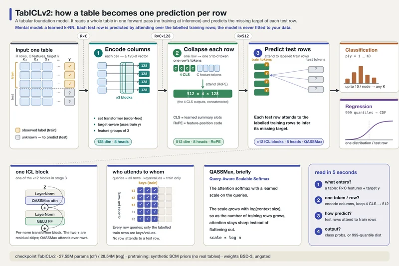
TabICLv2 is one of these in-context learners. Fitting takes seconds, and there are no hyperparameters to search. Under the label it is three transformers stacked, each answering a different question about the table, and it reads most easily in that order.

The first transformer reads down each column, one feature at a time. Its job is to turn a raw value into an embedding that knows what kind of number it is looking at, because the same digits mean different things in different columns. A 450 in a price column and a 450 in a postcode column are unrelated, and a model that only sees the number has no way to tell them apart. This stage is a set transformer: it treats a column as an unordered set of values, learns that column’s distribution, and gives each cell an embedding that reflects where the value sits within its own feature. So one 450 becomes “a fairly cheap item” and the other becomes “one particular area code”, from the same input number.

The second transformer reads across each row and collapses it to a single vector. After the first stage a row is a bag of per-feature embeddings, one for each column. A row is a set, and the standard way to summarise a set with a transformer is to add a few learned query tokens (the [CLS] tokens) and let them attend over the members. Here four [CLS] tokens per row pull together the parts of the row that matter, and their outputs are concatenated into one row vector. Whatever number of columns the row started with, it is now a single fixed-length vector standing in for the whole example.

The third transformer does the prediction, and this is where the in-context learning happens. No gradient descent runs at prediction time. Instead every unlabelled test-row vector attends over all the labelled train-row vectors, finds the training rows most like itself, and reads a label from them. The attention runs one way only, from test rows onto train rows, so the labelled examples inform the predictions but never the reverse. It is nearest-neighbours reasoning done with attention: the model looks at the examples whose answers it already knows, weighs them by similarity to the row in front of it, and predicts from them. The training set is fed in as context rather than baked into the weights, which is why you can point the model at a table it never saw in pretraining and get a prediction without training anything.

Two heads sit on top, one per task type. For classification, a hierarchical classifier assigns the label and works for any number of classes. For regression, the head does not emit a single number; it emits 999 quantiles, its estimate of the 0.1st percentile, the 0.2nd, and so on up to the 99.9th. That gives the full predictive distribution instead of a lone point estimate, so you can read a median and an honest interval around it.

Those 999 quantiles are trained with pinball loss, and it is worth seeing why that loss produces quantiles at all. For a target quantile, say the 90th percentile, pinball loss charges a different price for being too low than for being too high. Undershoot the true value and you pay 0.9 × error; overshoot and you pay only 0.1 × error. That asymmetry pushes the prediction upward until about 90% of the real values fall below it, which is the definition of the 90th percentile. Apply the same rule to all 999 targets at once and each output settles at its own slice of the distribution. The name comes from the shape of the loss plotted against the error: a lopsided V, steep on one side and shallow on the other, like the tilt of a pinball table. At the median it is symmetric and reduces to plain mean-absolute error.

The details that let v2 scale where v1 stalled are in the paper: a query-aware rescaled softmax (QASSMax) so attention does not fade over long context, feature grouping that breaks the symmetry between columns, and target embeddings injected early.

Three properties make it the right audit target: small, open, and reproducible at once. The weights are on HuggingFace under BSD-3 with no gating and no click-through licence; pip install tabicl and it runs. Loading the two checkpoints and counting gives exactly 27,552,258 parameters for the classifier and 28,544,991 for the regressor, so “about 28M” comes from counting the tensors in the downloaded checkpoints. That is roughly a quarter of t0-alpha’s size, for a model that tops tuned GBDTs. Its main rivals do not share the property in full: the TabPFN line (Prior Labs) publishes weights under a non-commercial licence with a licence-acceptance step in its tooling, and TabFM (Google Research) shipped weights under a non-commercial licence with no paper at all. Open weights matter here for the same reason as before: anyone can rerun the evaluation and check the claim.

TabICLv2 is also pretrained purely on synthetic data, generated from random structural causal models. No real-world table enters pretraining, so no benchmark dataset can leak into it. The contamination section below sets this against the newer models that add real pretraining data.

Trying one on your own table

The practical surface is scikit-learn. TabICLv2 installs with pip install tabicl, downloads its checkpoint from HuggingFace on first use, and accepts a pandas DataFrame with categorical columns and missing values as-is:

from tabicl import TabICLClassifier # TabICLRegressor for regression clf = TabICLClassifier() # defaults are fine: no hyperparameter search clf.fit(X_train, y_train) # seconds: stores context, no gradient training proba = clf.predict_proba(X_test) # one forward pass
It runs on CPU for small tables, but the speed numbers in this post are GPU numbers; a single consumer GPU is the intended home. The working range is bounded: TabICLv2 was pretrained on tables of roughly 300 to 48,000 training rows, the benchmark below tops out at 150,000 rows, and my regime analysis later in the post shows accuracy degrading on very wide tables (over ~100 features). Inside that envelope, the model won 86–88% of datasets against the tuned trees in my regime analysis and fits in seconds; outside it, the trees section below is where to look.

The benchmark, and the part I verified myself

TabArena is 51 curated datasets spanning binary classification, multiclass, and regression, from 748 to 150,000 rows and 5 to 1,777 features. Every method is evaluated with repeated cross-validation (9–30 splits per dataset), models are compared with task-appropriate metrics (ROC-AUC, log-loss, RMSE), and the aggregate is an Elo rating: each pairwise per-task comparison is a “game”, and the scale is anchored so a default RandomForest sits at 1000 and a 400-point gap means 10:1 win odds. It is a living benchmark; methods and results get added continuously.

Before quoting anyone’s Elo I wanted to know I could recompute it. TabArena publishes its per-split results as downloadable artefacts, so I ran the maintainers’ own aggregation pipeline locally over those artefacts, with their official constants (200 bootstrap rounds, imputed methods excluded), and diffed my board against the CSV behind tabarena.ai. All 69 methods matched, 67 of 69 to within ±1 Elo, and the ordering of the top 30 came out identical (Spearman ρ = 0.99998 across the board). That check validates the scoring and aggregation code, the same role the Seasonal-Naive match played in the t0 post. It does not validate any model’s own predictions; that is what the re-run is for.

The two rows that differed by more than a point were tuned TabM configurations (+4 and +5 Elo); all three TabM variants’ runtime columns shifted as well, because TabM’s results artefact was updated after the current website snapshot was published. The benchmark is updated continuously, so everything below is pinned to the 2026–07–15 snapshot.

The recomputation also showed that Elo is pool-dependent. My first attempt included the imputed methods the website excludes, and every rating shifted by 10–30 points. The per-dataset metrics in the artefacts are the pool-independent numbers; Elo summarises them relative to whichever pool you score.

The standings

All Elo figures below are from the official board (snapshot 2026–07–15), which I recomputed to ±1 Elo from the published artefacts. These are full-protocol numbers (9–30 splits per dataset); my own run uses the official Lite protocol (1 split per dataset), so it appears as a separate comparison under the table rather than a row inside it.

Restricting the whole pool to the Lite splits and merging in my fresh run: official TabICLv2 scores 1575 there and mine 1559, ranks 5 and 6 on the same board. The reproduction section above has the per-task numbers.

First, every single model above the best GBDT configuration is a tabular foundation model; the only non-FM entries above it are the AutoGluon ensemble pipelines. LightGBM with full tuning and post-hoc ensembling reaches 1432; TabICLv2 with no tuning at all sits 158 Elo above it, and the gated TabPFN line higher still. On this board, at these dataset sizes (748 to 150k rows), the accuracy frontier belongs to the foundation models. I did not expect the margin to be that wide.

Second, the serving cost complicates the usual defence of trees (“sure, but they’re cheap”). TabICLv2’s median predict time is 0.38 s per 1,000 rows, faster than tuned-and-ensembled LightGBM (2.64) and in the same range as tuned CatBoost. Its median fit time, 4 s per 1,000 rows, is roughly a hundred times shorter than the tuned GBDT protocols, because fitting is a single forward pass with no hyperparameter search. One caveat: the foundation models run on a GPU and the trees on CPU, so the dollars-per-row comparison depends on your infrastructure, and default CatBoost at 0.08 s/1K on a CPU is still the cheapest sane option on the board. For scale: my entire 51-dataset TabICLv2 sweep, on-demand A10G, cost $2.

Third, TabFM sits at the top, 98 Elo clear of the next entry (the AutoGluon pipeline) and 123 clear of the next single model, and it joined the board on 2026–06–30, two weeks before I wrote this. The audit came out better than I expected on data and worse on documentation. Its pretraining is entirely synthetic, from structural-causal-model priors like TabPFN’s and TabICL’s, so benchmark contamination is ruled out by construction for it too. What it lacks is a paper: there is no technical report, no published parameter count, and the weights carry a non-commercial licence the README does not mention Christoph Molnar’s write-up. An independent fold-matched re-test still found it ahead of tuned XGBoost. I report its numbers and mark it as not-independently-run in the chart; the 123-Elo gap looks real, but nobody outside Google can yet say why it works.

Pasting the table into a frontier LLM, measured

I also put a number on the serialise-and-prompt line: Claude Opus 4.8 given each dataset as text, with 64 labelled example rows in the prompt, then batches of test rows to predict and per-class probabilities requested as structured output. To keep it affordable this is a reduced protocol: 50 subsampled test rows per dataset, at most 32 columns shown, one batched API run over all 51 datasets. The subsample makes each per-dataset score noisy, so read the aggregate, not any single row.

The aggregate is one-sided. Two of the 51 datasets returned too few usable predictions to score; on the remaining 49, the LLM beats TabICLv2 on 6 and the best tuned-and-ensembled GBDT on the same 6, with a median error 57% higher than TabICLv2’s. It wins on churn, credit and blood-donation tables, where column names carry real-world meaning an LLM can exploit. It loses badly on app-permission vectors and sensor and physical-process data, where the table is pure pattern and the language prior contributes nothing. “Tabular LLM” as a phrase invites conflating the two model classes; on this protocol the 28M-parameter table-native model won 43 of 49 datasets, and it serves a thousand rows for a fraction of a GPU-second where the prompted LLM cost me about $1.50 per thousand predictions.

What tuning does to the GBDT baselines

The first objection any GBDT partisan will raise is tuning: nobody ships default LightGBM, so a board that ran the trees on defaults would oversell the foundation models. TabArena already contains the answer, because it runs every GBDT at three budgets: default config, tuned (a real search, hours of compute), and tuned + post-hoc ensembled.

Tuning is worth a lot for LightGBM and XGBoost, on the order of 200 Elo, which is most of the distance between “mid-table” and “best tree on the board”. CatBoost is the exception: its defaults are already within 47 Elo of its fully tuned-and-ensembled self, which matches its reputation and makes default CatBoost the strongest cheap baseline here (1370, on a CPU, at 0.08 s/1K to serve).

So the objection was priced in before I arrived, and the conclusion survives it: give the trees their full tuning budget and ensembling, and the untuned foundation model still sits 150+ Elo above them. (In time series I found the opposite — proper tuning halved the foundation models’ apparent edge. Here it doesn’t come close to closing the gap.)

The aggregate masks a regime split that says where a tree is still the right choice. Per dataset, against the best of the three tuned-and-ensembled GBDTs, TabICLv2 wins 40 of 51. The eleven losses cluster in two places.

The first is dimensionality: of the six datasets with more than 100 features, the foundation model wins exactly one. Bioresponse (1,776 features), hiva_agnostic (1,617), QSAR-TID-11 (1,024), kddcup09 (212) and MIC (111) all go to the trees. Below 100 features the FM wins 86–88% of datasets.

The second is scale with high-cardinality categoricals: the single largest tree win on the board is Amazon_employee_access (a 25% error gap), the classic dataset of exactly that shape, and the FM’s win rate slides from 89% under 3,000 rows to 64% above 20,000. Task type barely matters (77–85% across binary, multiclass, regression). Six datasets is a thin cell to generalise from, so read the dimensionality finding as a strong hint rather than a law. Still: if your table is wide or your categoricals are wild, reach for the tuned GBDT first.

Contamination: the cleanest-provenance models are being out-scored

Benchmark contamination was the axis my time-series audit turned on, and it matters here too, with a different shape: the models with the cleanest data provenance are the ones being out-scored.

TabICLv2 and the original TabPFN line are pretrained on synthetic data only. There is nothing to leak: no benchmark table can be in a pretraining corpus that contains no real tables, so for these models contamination is ruled out by construction.

The reason the topic is live anyway is that accuracy gains increasingly come from adding real data. RealTabPFN-2.5 continues pretraining on “a curated corpus of 43 real-world tabular datasets sourced from OpenML and Kaggle”, and its report describes the strongest dedup pipeline I found anywhere in this audit: dataset IDs, names, shapes, feature names, row and column hashes, manual metadata inspection, “deduplicated against all internal benchmarks and the full TabArena suite” Real-TabPFN paper; TabPFN-2.5 report, Appendix C. TabDPT goes further down the real-data road: it is pretrained on 123 OpenML datasets outright, and TabArena’s datasets come from OpenML, which is exactly the overlap a recent ensembling paper flags as a contamination concern, noting its reported gains “should be read as upper bounds”. I have no reason to disbelieve any specific dedup pipeline; I also cannot verify one, and the incentive gradient points one way: real data buys Elo, and the burden of proving it bought Elo cleanly rests on self-declared dedup. That is the same epistemic position as the self-declared “No” leakage flags on GIFT-Eval.

The provenance map of the board, from the audit:

The practical reading, for now: if you want a number you can fully trust on your own data, the synthetic-only models give you the cleanest evidential position, and TabICLv2 is the strongest of them with unrestricted weights. If you want the last 100–200 Elo, you buy models whose training data you have to take on trust, or run your own held-out evaluation.

Hybrid headroom: oracle ceilings and a deployable router

Complementary models can be routed between, and TabArena’s published artefacts allow something my time-series analysis couldn’t: they contain per-split validation errors alongside the test errors, so I can score both the oracle router (pick the better model per dataset using test error, a ceiling, since it cheats) and a deployable one (pick using validation error, which a real system has). No model runs; this is pure arithmetic on the published per-split results, scored with the board’s own Elo machinery.

One scale note: these Elo values are computed in my own pool (all 78 published methods plus the routers, imputed methods included), so the absolute numbers sit a few points off the website’s board — TabICLv2 is 1571 here versus 1590 there. Comparisons within the table are like-for-like.

The complementarity is real, and it includes the trees. An oracle that picks per dataset between TabICLv2 and tuned LightGBM reaches 1674, a +103 gain over TabICLv2 alone — from a partner that sits 160 Elo below it. TabICLv2 wins on 42 of the 51 datasets head-to-head, and the other nine are worth that much. The FM+FM oracle is bigger still: 1707, above everything on the board except the unaudited TabFM.

The deployable router works, but only between foundation models. Picking between TabICLv2 and TabPFN-2.6 by validation error scores 1645, above both of its members, recovering roughly half the oracle headroom with nothing an oracle would need. Routing between complementary models beats the best single model, using only information you have at deployment time.

The same router backfires across the FM/GBDT divide. Val-picking between TabICLv2 and tuned LightGBM lands at 1534, below just always using TabICLv2. The oracle says +103 of headroom exists there; validation-based selection not only fails to capture it, it lands 37 Elo below always running TabICLv2, presumably because the two model families’ validation errors are not comparable (the GBDT’s bagged internal validation estimates look optimistic next to the FM’s). I’m flagging the mechanism as a guess; the direction of the result is measured. If you want the tree’s nine datasets, you need a better selection signal than raw validation error.

What I take from this

A 28M-parameter open model, pretrained on no real data at all, reproduced its public benchmark standing on my hardware to within bootstrap noise (16 Elo on identical splits; median per-task difference 0.08%) for $2 of GPU time, and the board it sits on shows every tuned, ensembled gradient-boosted tree configuration at least 158 Elo below it. The part I’d stake most on is the evidential position: open weights, synthetic-only pretraining, and a scoring pipeline I recomputed myself end to end. What I would not yet claim is the top of the board: TabFM’s provenance is unaudited, the TabPFN line is gated, and my own run covered one split per dataset rather than the full protocol.

If you’re holding a table today, the regime map above turns into a short decision rule. Under a hundred features and modest row counts, TabICLv2 zero-shot is the strongest thing you can run with fully open weights, and it fits in seconds. Wide tables and wild categoricals still belong to a tuned GBDT. If you can serve two models and your candidates are both foundation models, validation-picking between them added accuracy in my measurement; across the FM/tree divide it subtracted accuracy, so avoid it there.

One row remains open: I have not yet independently re-run a TabPFN model. The next experiments I’d run: that TabPFN-2.6 re-run on the same Lite splits, and a weighted FM+GBDT ensemble from TabArena’s cached predictions to see how much of the oracle’s +103 a real combination recovers on the high-dimensional datasets the router can’t reach.

Disclaimer: The views and opinions expressed in this article are my own and do not represent those of my employer or any affiliated organizations. The content is based on personal experience and reflection, and should not be taken as professional or academic advice.

📚References

Erickson, N., Purucker, L., Tschalzev, A., Holzmüller, D., Desai, P. M., Salinas, D., and Hutter, F. (2025). TabArena: A Living Benchmark for Machine Learning on Tabular Data. Introduced TabArena, the continuously maintained benchmark used throughout this article, including its curated datasets, repeated evaluation protocol, model comparisons and Elo-based leaderboard.
Qu, J., Holzmüller, D., Varoquaux, G., and Le Morvan, M. (2026). TabICLv2: A Better, Faster, Scalable, and Open Tabular Foundation Model.Introduced TabICLv2, the approximately 28-million-parameter open tabular foundation model independently evaluated in this article, and describes its synthetic pretraining, architecture and scaling improvements.
Hollmann, N., Müller, S., Eggensperger, K., and Hutter, F. (2023). TabPFN: A Transformer That Solves Small Tabular Classification Problems in a Second.Established the use of pretrained transformers and in-context learning for tabular prediction, using synthetic datasets generated from structural causal model priors.
Hollmann, N., Müller, S., Purucker, L., Krishnakumar, A., Körfer, M., Hoo, S. B., Schirrmeister, R. T., and Hutter, F. (2025). Accurate Predictions on Small Data With a Tabular Foundation Model. Presents the modern TabPFN generation for small-to-medium tabular datasets and demonstrates that a pretrained foundation model can compete with extensively tuned conventional methods without dataset-specific parameter training.
Google Research. (2026). Introducing TabFM: A Zero-Shot Foundation Model for Tabular Data. Introduces TabFM, the highest-ranked model discussed in the article, and describes its zero-shot classification and regression approach, in-context inference and synthetic structural-causal-model pretraining.